Overview
The January 2025 Los Angeles wildfires burned through steep chaparral canyons directly into densely populated residential areas of the Wildland-Urban Interface (WUI). This project frames post-fire structural damage assessment as a semantic segmentation task: given multispectral satellite imagery, topographic data, and building footprints, can we predict which structures were destroyed — before field inspections are complete?
We train and evaluate across two fire events — the Palisades Fire and the Eaton Fire — to improve generalizability and double the available training data.
Target users: LA County Department of Regional Planning, utility providers, environmental resilience agencies.
Problem & Motivation
Civic agencies currently wait for labor-intensive field inspections before allocating rebuilding resources, estimating insurance liabilities, or deploying soil stabilization teams. A pixel-level damage prediction map from satellite imagery provides immediate, actionable intelligence for post-disaster zoning and debris removal prioritization.
Key Technical Challenges
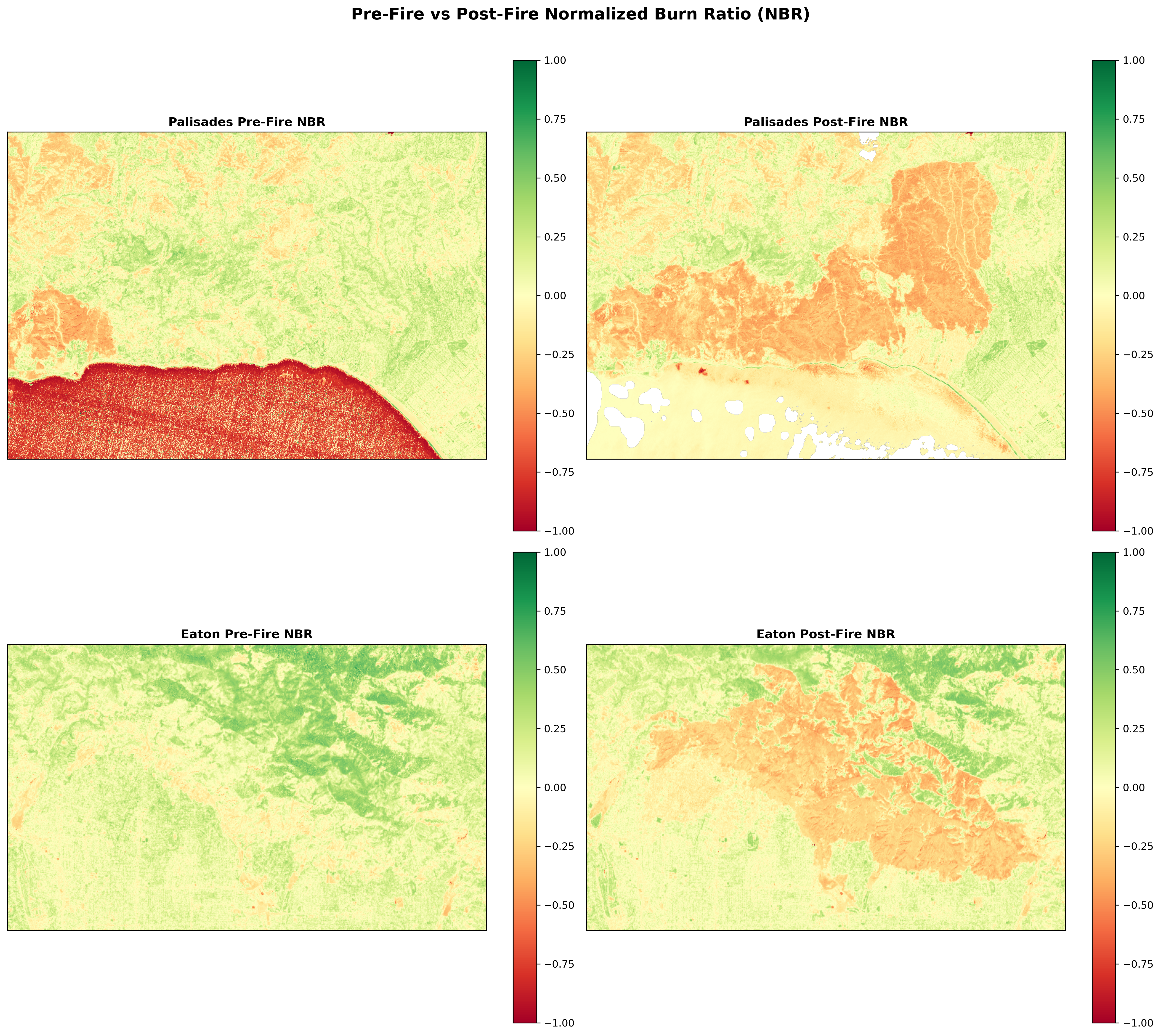
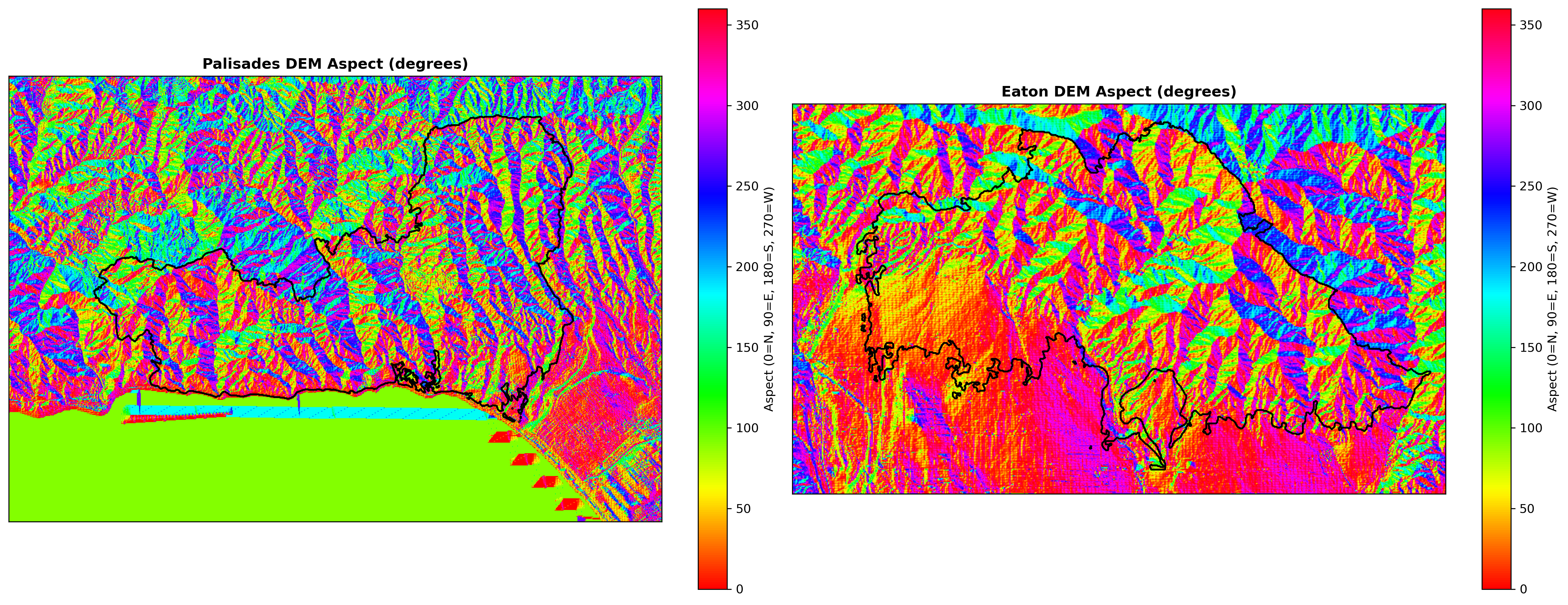
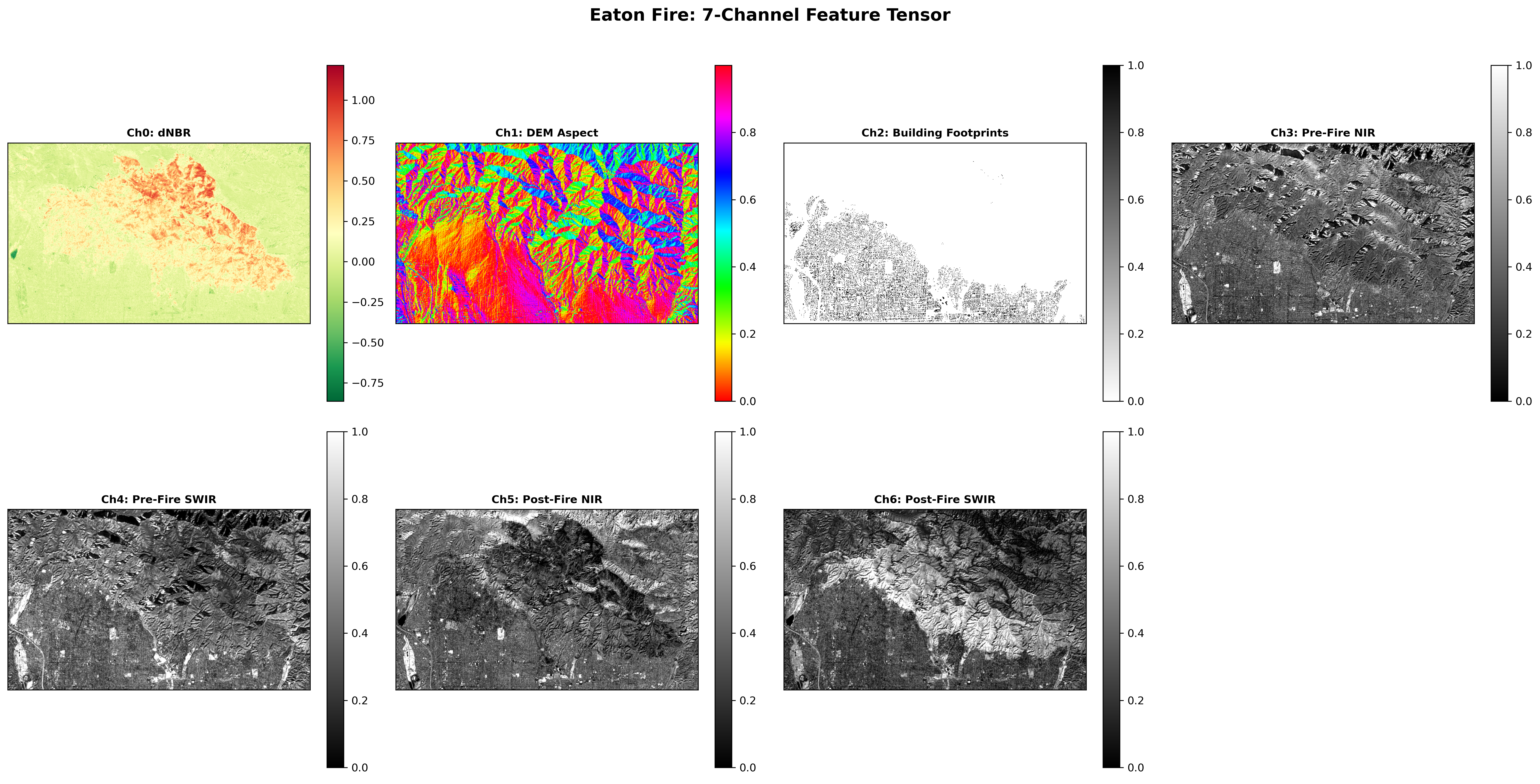
1. Topographic shadowing — In January, the sun sits low in the southern sky. Steep north-facing canyons cast deep shadows that mimic severe burn spectral signatures. DEM-derived aspect is fed explicitly into the model to distinguish shadow artifacts from genuine burns.
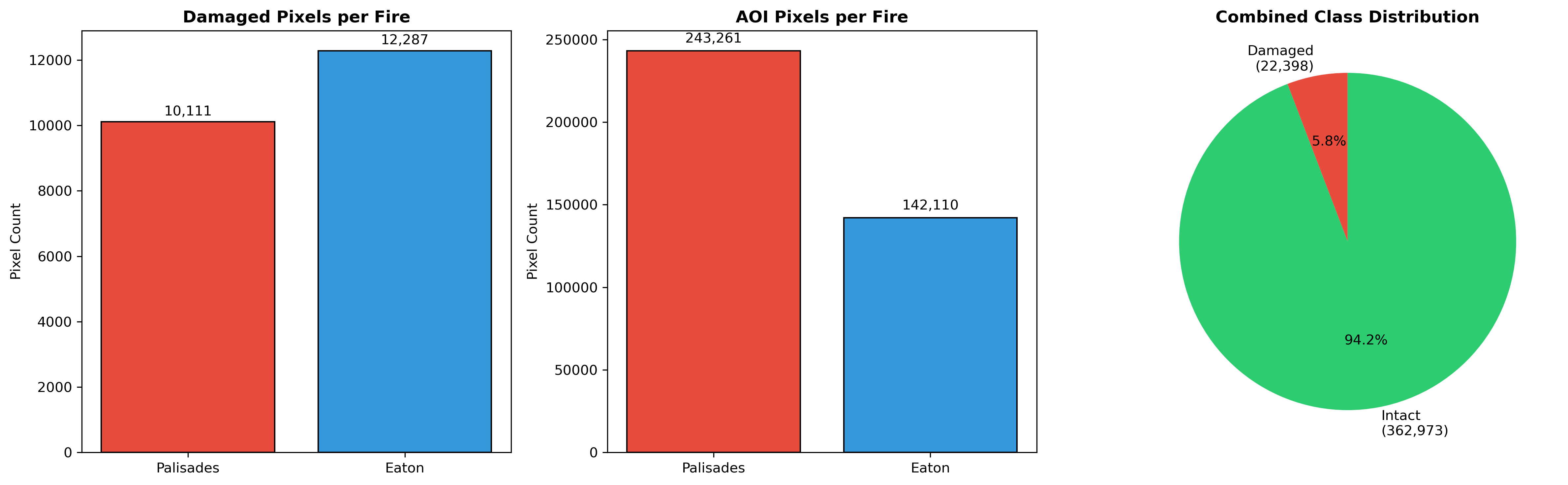
2. Class imbalance — Destroyed buildings represent ~5.8% of combined fire perimeter pixels (16.2:1 negative-to-positive ratio). Combined Dice Loss + Focal Loss addresses this.
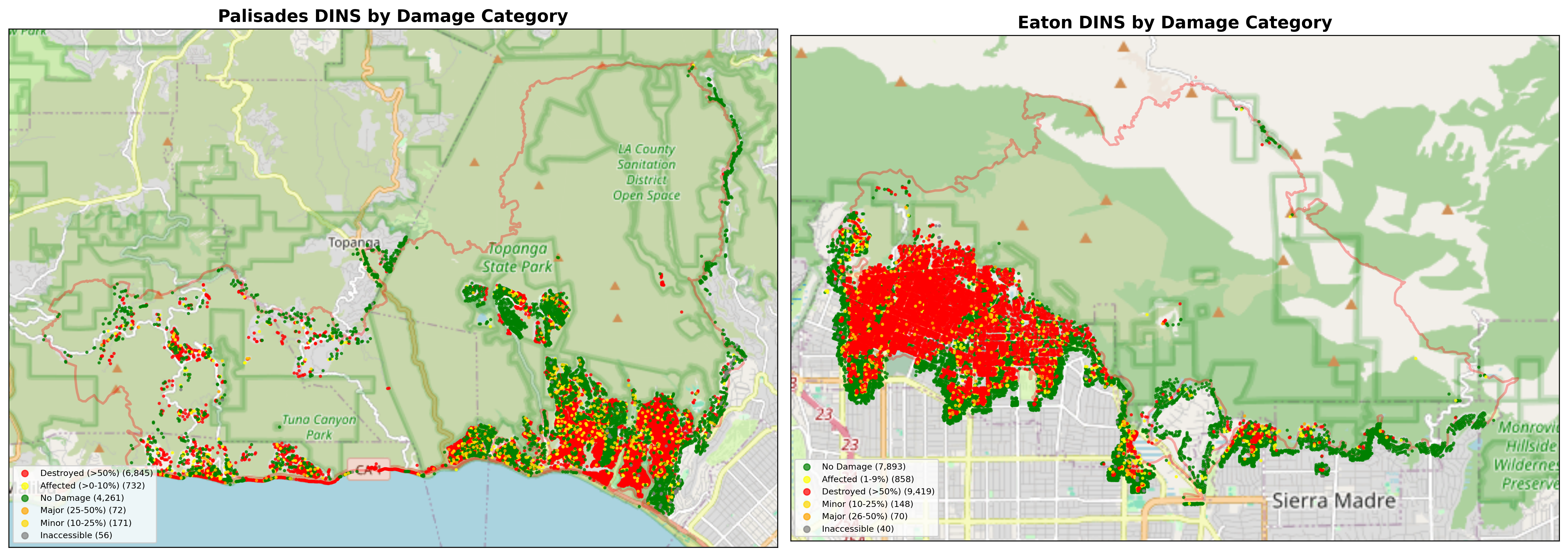
3. Target leakage prevention — dNBR is an input feature, not a label source. Ground truth comes exclusively from CAL FIRE DINS field inspections, ensuring the model learns predictive relationships rather than circular spectral thresholds.
Study Area
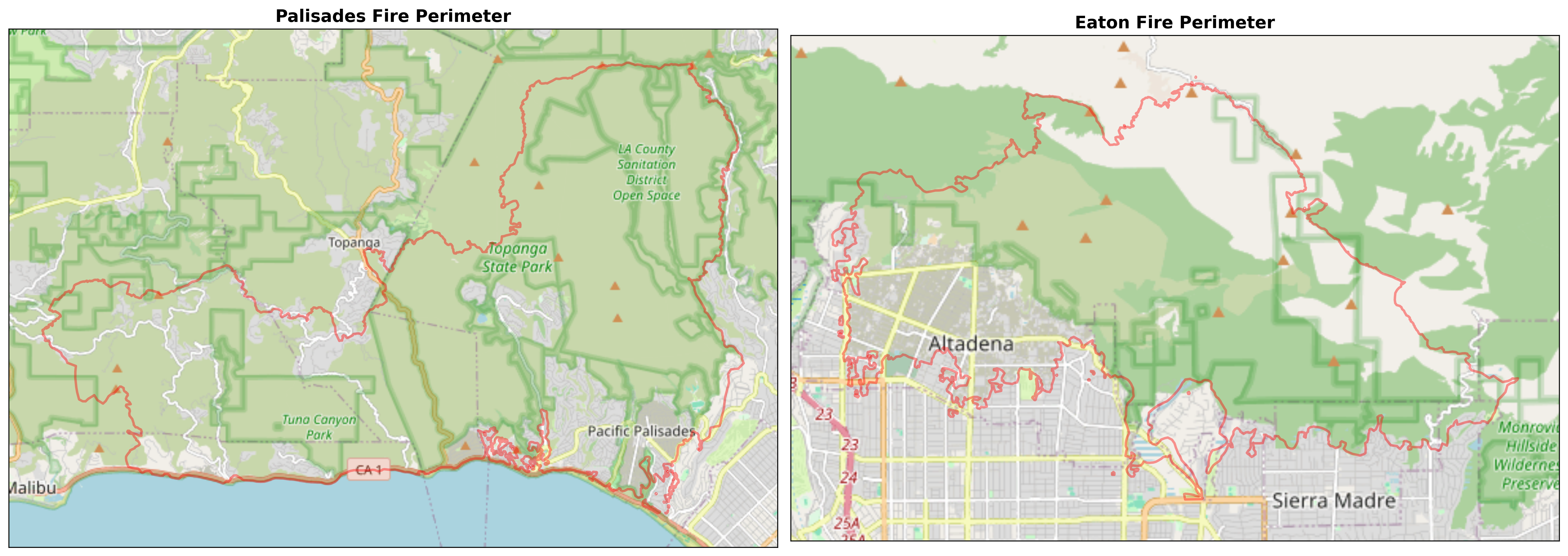
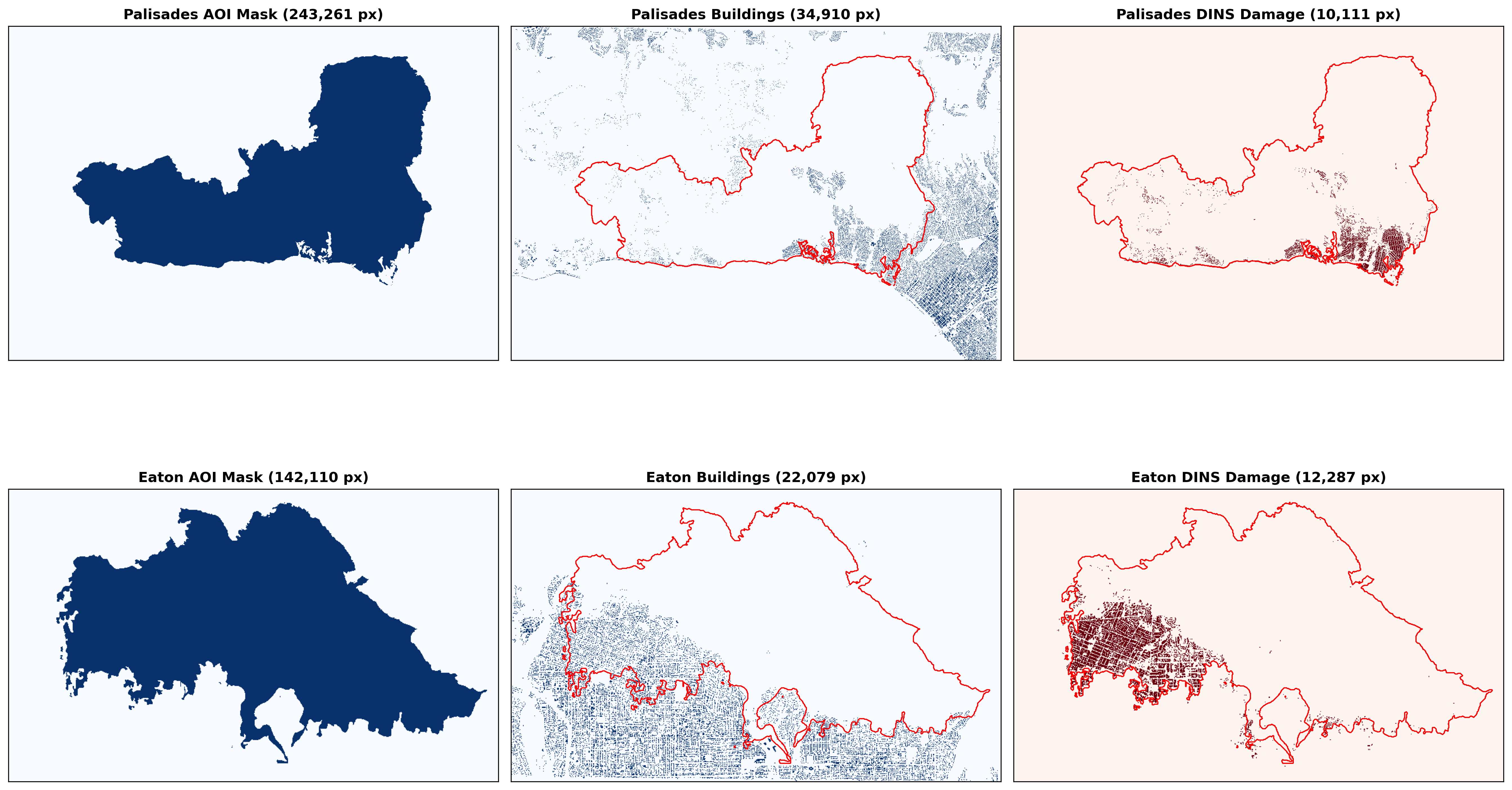
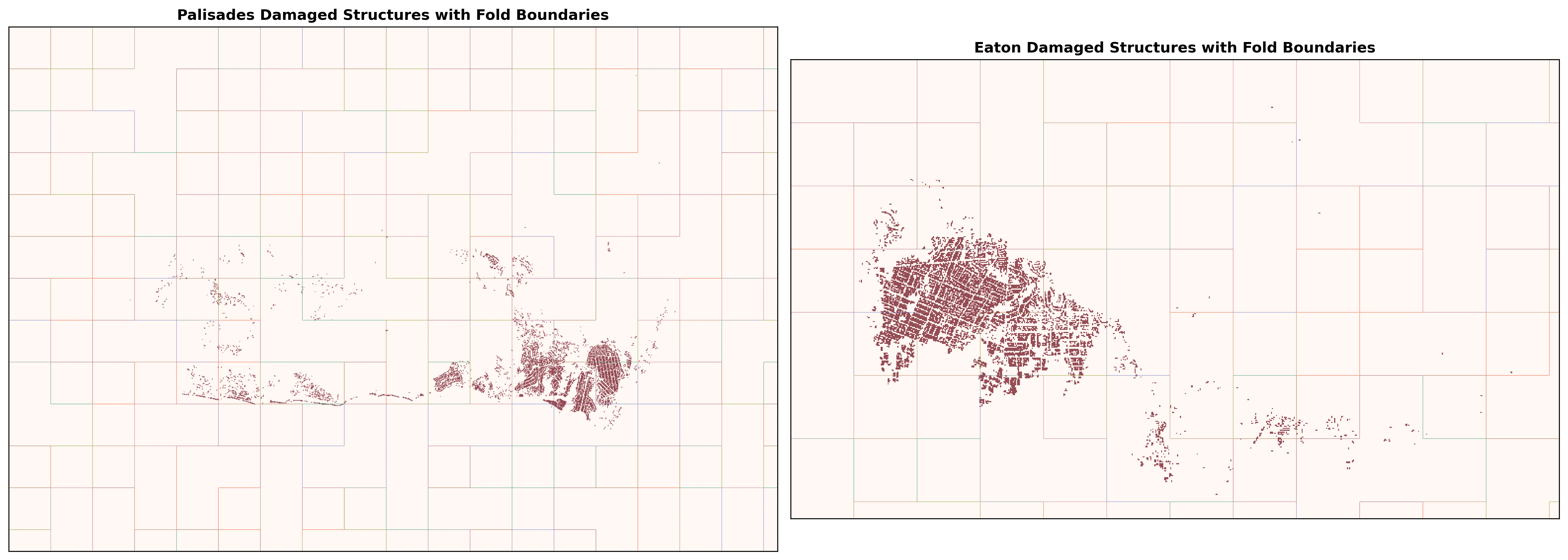
Both fires occurred during the same January 2025 weather event and were processed through an identical pipeline. Using two geographically distinct fires — Palisades in the coastal Santa Monica Mountains, Eaton in the inland San Gabriel foothills — exposes the model to different topographic conditions and nearly doubles training data compared to a single-fire setup.
| Palisades |
Pacific Palisades / Malibu |
243,261 |
10,111 |
4.16% |
| Eaton |
Altadena / Pasadena |
142,110 |
12,287 |
8.65% |
| Combined |
|
385,371 |
22,398 |
5.81% |
Data
| Pre/Post-fire optical (NIR, SWIR) |
Sentinel-2 L2A via STAC API |
20 m |
| dNBR (delta Normalized Burn Ratio) |
Computed from Sentinel-2 |
20 m |
| Topographic aspect |
USGS 3DEP 10m DEM |
Resampled to 20 m |
| Building footprints |
Microsoft US Building Footprints |
Rasterized to 20 m |
| Ground truth labels |
CAL FIRE DINS field inspections |
Point → 15 m buffer → raster |
| AOI boundary |
NIFC FIRIS fire perimeters |
Vector |
Temporal windows: Pre-fire: 2024-12-01 – 2025-01-06 · Post-fire: 2025-02-01 – 2025-02-28
Preprocessing
Sentinel-2 L2A is used because atmospheric correction is required when comparing imagery across two dates — without it, atmospheric variation mimics spectral change. Scenes are ranked by cloud cover and the lowest-cloud acquisition is selected per fire; where a fire straddles two tiles (Eaton), all tiles from the best date are mosaicked. Pixels are cloud-masked using the SCL layer before any spectral computation.
The pre-fire window closes one day before ignition; the post-fire window starts February 1 to allow active fire and smoke to clear.
Aspect is chosen over elevation or slope because it determines solar illumination angle: north-facing slopes in Southern California both retain more moisture and are most likely to be in shadow during January acquisitions, so aspect is the variable most confounded with burn severity at this location and season.
Modeling Approach
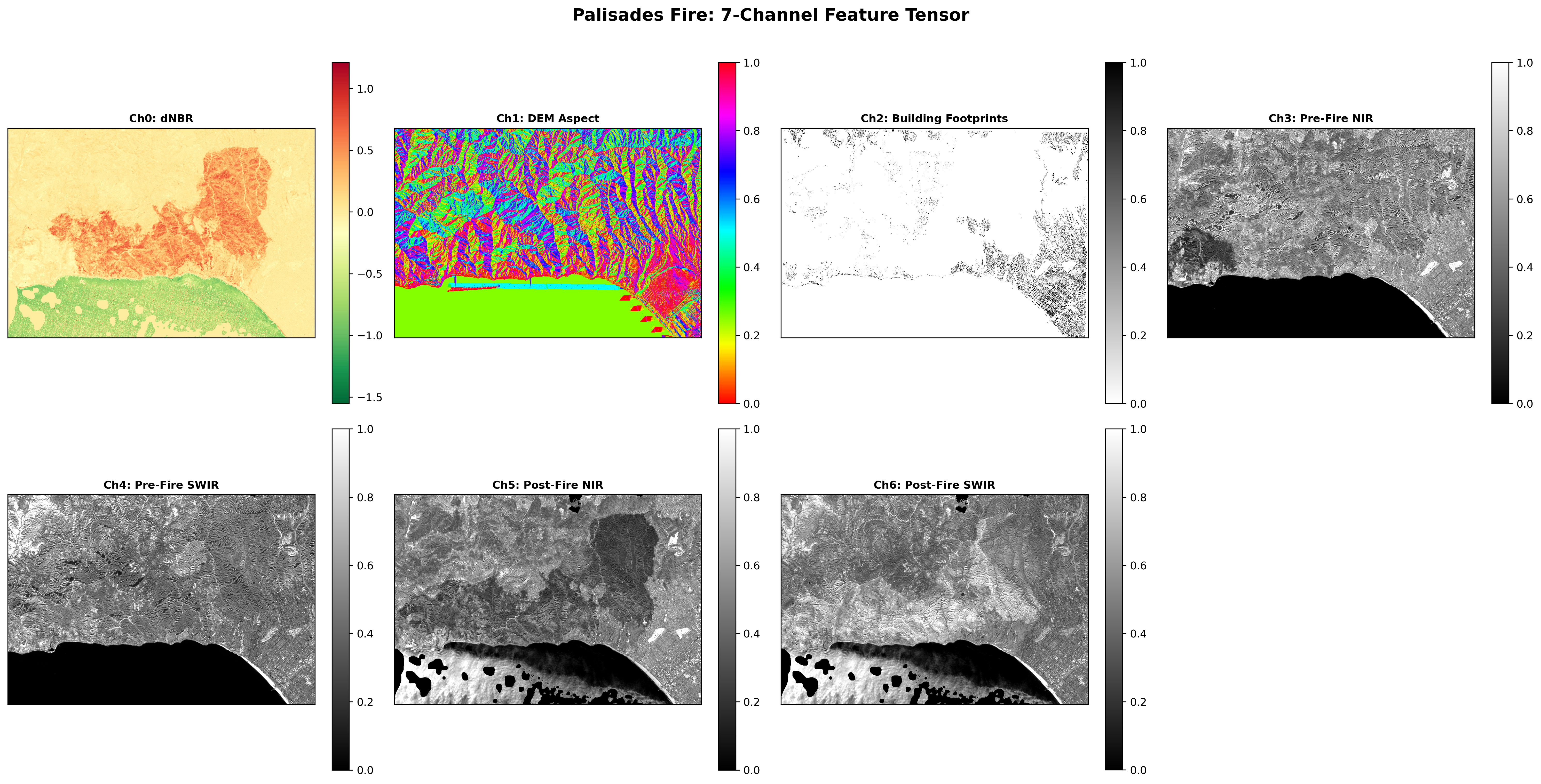
The input tensor is a 7-channel stack per pixel:
\[\mathbf{X} = [\text{dNBR},\ \text{DEM Aspect},\ \text{Building Footprints},\ \text{Pre-NIR},\ \text{Pre-SWIR},\ \text{Post-NIR},\ \text{Post-SWIR}]\]
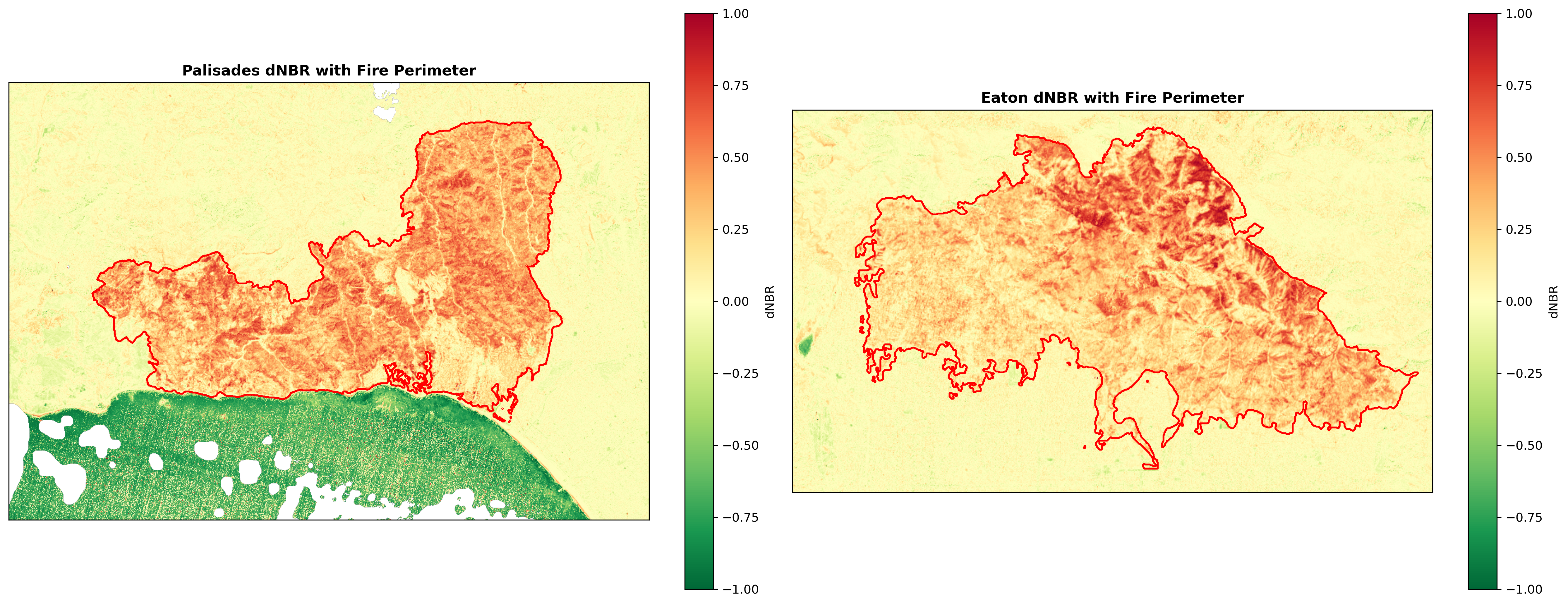
Raw pre- and post-fire NIR/SWIR bands are included alongside dNBR because dNBR encodes only the relative change between dates, discarding absolute reflectance context. Including the underlying bands lets the model learn that a given dNBR value means different things over bare soil versus dense forest.
Spatial K-Fold Cross-Validation
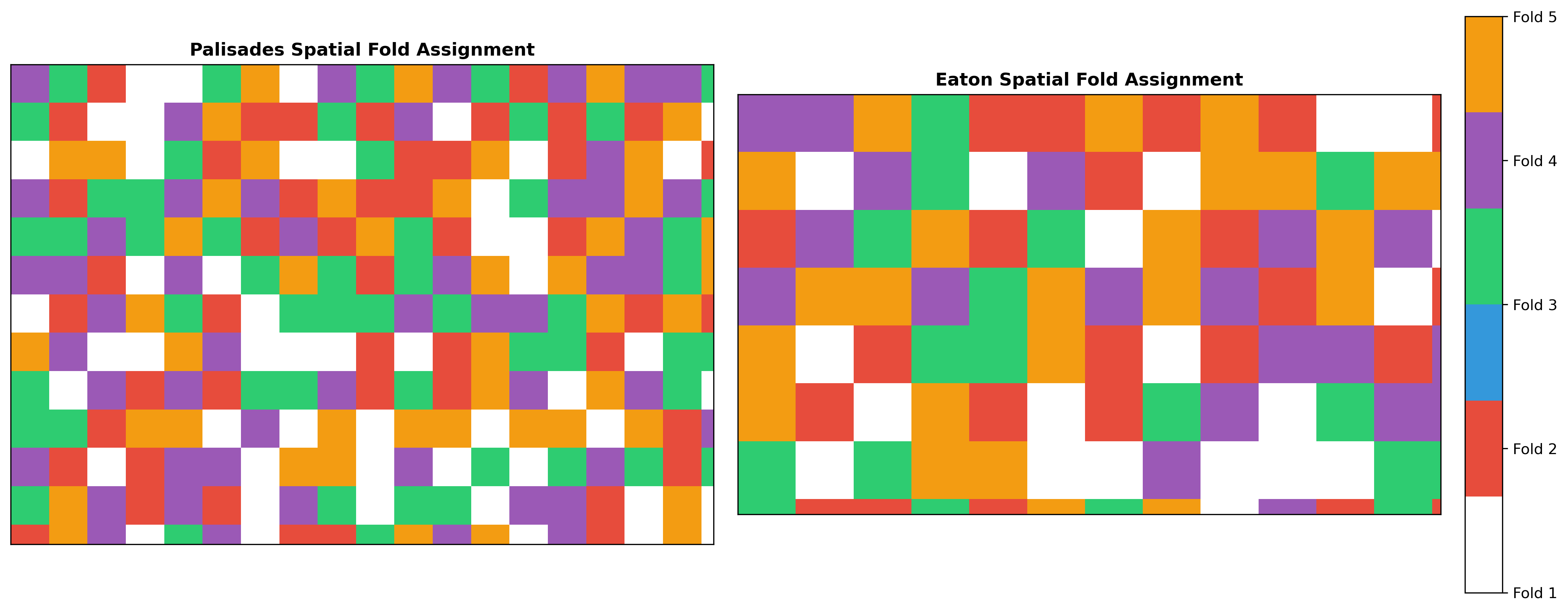
Fire damage clusters spatially — entire blocks burn together. A random pixel-level split would place test pixels immediately adjacent to training pixels, producing inflated metrics via spatial interpolation rather than genuine generalization. Spatial K-Fold assigns whole 64×64 pixel blocks to folds, ensuring train and test regions are geographically separated. Blocks are stratified by damage presence because most blocks contain no damage at all — without stratification, some folds would have almost no positive labels.
Baseline: Random Forest
A pixel-wise Random Forest treats each pixel independently and establishes a lower bound: if the U-Net cannot beat it, spatial context adds no value. class_weight="balanced" is required because an unweighted classifier maximizes accuracy by predicting “no damage” everywhere, achieving 94% accuracy with zero recall on the damage class.
Training: 5-fold spatial cross-validation · class_weight="balanced" · Evaluated on F1-Score (positive damage class only)
Primary: Topographically-Aware U-Net
The U-Net encoder–decoder learns that a damaged pixel appears in a cluster with high dNBR, a building footprint, and a specific aspect — a spatial pattern the pixel-independent Random Forest cannot represent. Skip connections preserve fine structural boundaries that would otherwise be lost during downsampling.
Architecture: Input (64, 64, 7) → 3-level Encoder (Conv + BatchNorm + ReLU) → Bottleneck → Decoder with skip connections → Binary sigmoid output
Regularization: SpatialDropout2D drops entire feature maps rather than individual activations. For convolutional layers, adjacent activations are highly correlated, so standard Dropout has little effect; dropping whole channels forces the network to learn redundant representations across channels. This was the primary fix for the overfitting observed in the earlier single-fire model.
Data augmentation: Random horizontal/vertical flips and 90° rotations are valid for nadir satellite imagery, which has no canonical orientation. Discrete 90° steps are used to avoid interpolation artifacts in the label masks.
Loss functions: - Dice Loss — optimizes overlap directly; prevents the model from collapsing to predicting all-negative at 5.8% prevalence - Focal Loss (alpha=0.80, gamma=3.0) — alpha upweights the positive class; higher gamma than default applies stronger down-weighting to easy background pixels - Combined Loss — Dice operates at the patch level (global shape), Focal at the pixel level (local precision); combining both provides complementary supervision
Training details: Batch size 16 · Max 50 epochs · Early stopping patience 10 · ReduceLROnPlateau patience 5 · Positive-class patch 2× oversampling
Results
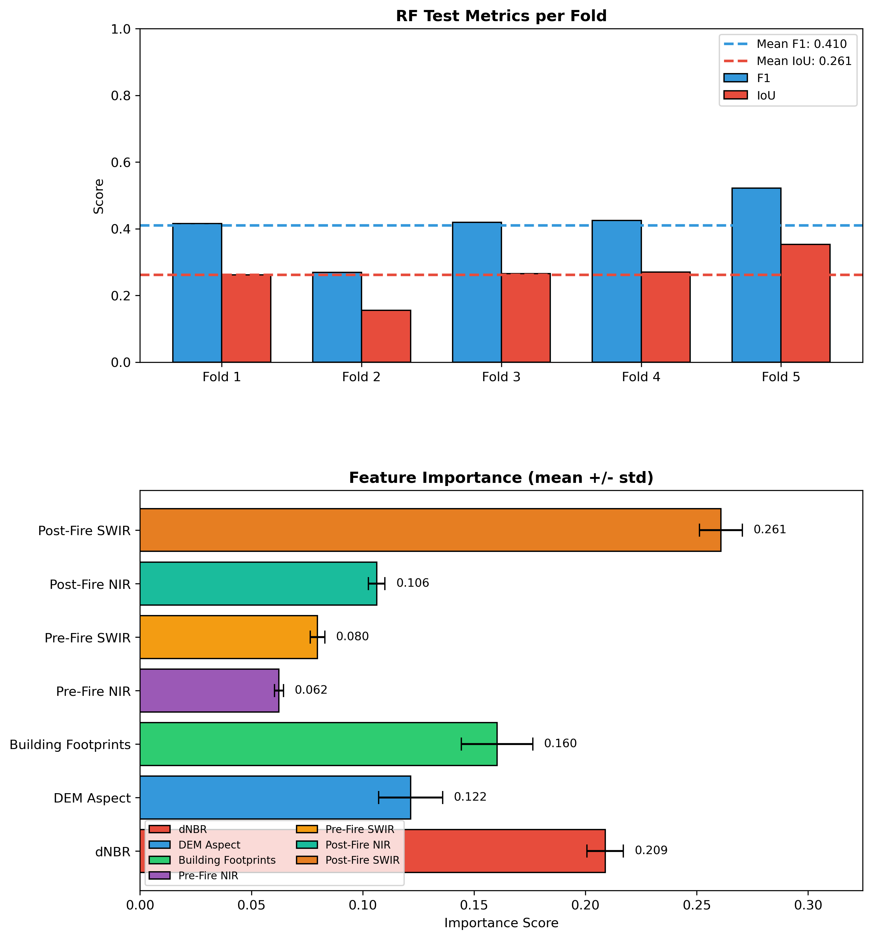
| Random Forest (baseline) |
0.4101 ± 0.0810 |
0.2611 ± 0.0629 |
| Topographically-Aware U-Net |
0.6532 ± 0.0469 |
0.4868 ± 0.0520 |
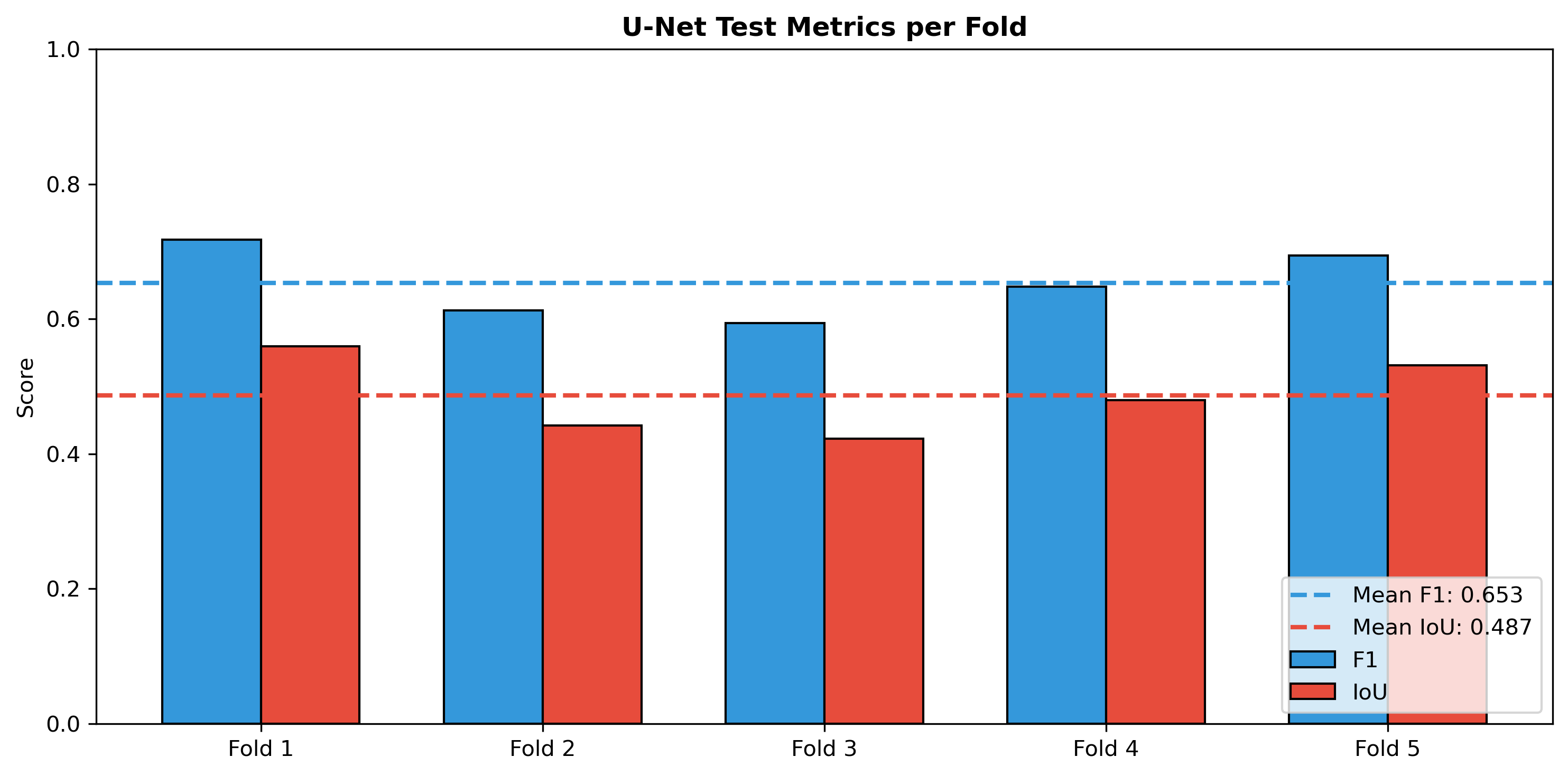
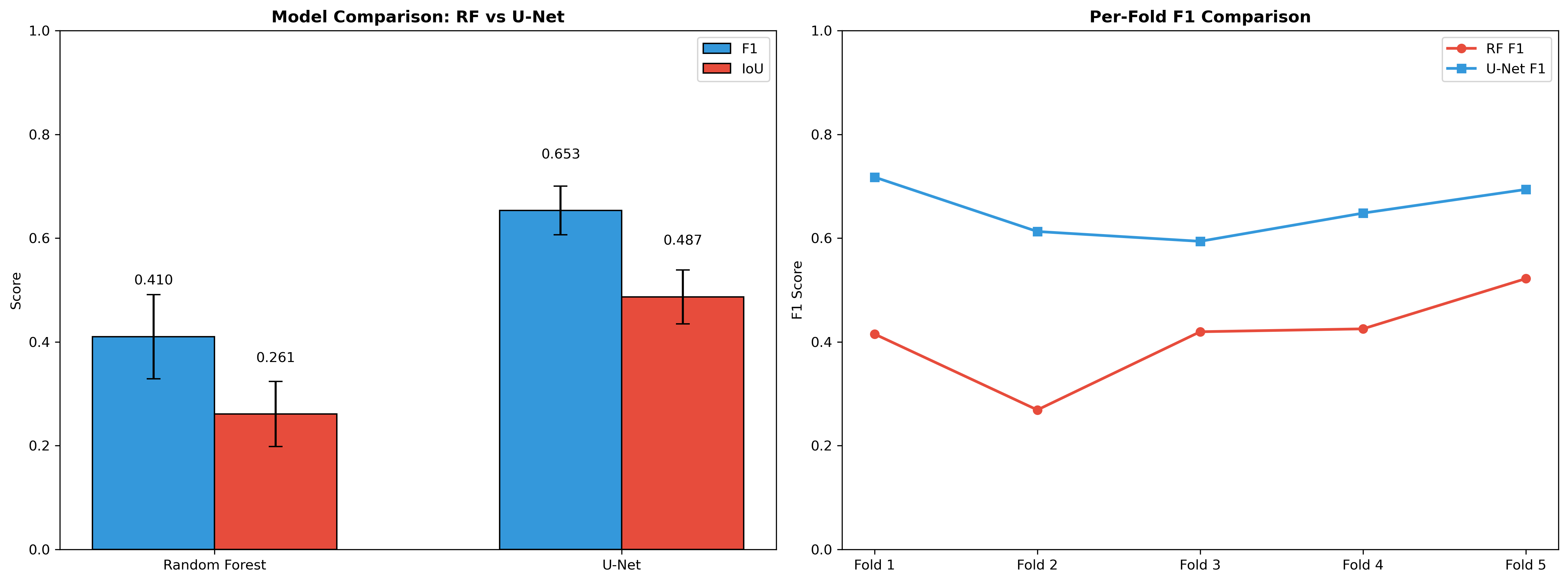
The U-Net improves F1 by +0.24 and IoU by +0.23 over the Random Forest baseline. The lower standard deviation (0.047 vs. 0.081) indicates more consistent generalization across folds. The model has confirmed predictive signal (F1 ≥ 0.50) but has not yet reached the operational utility threshold (F1 ≥ 0.70).
F1 is the primary metric because accuracy is dominated by the 94% majority (undamaged) class — a model predicting “no damage” everywhere would score 94% accuracy while detecting nothing. F1 measures precision and recall on the damage class only.
Random Forest Feature Importance
| Post-Fire SWIR |
0.2609 ± 0.0096 |
| dNBR |
0.2089 ± 0.0082 |
| Building Footprints |
0.1603 ± 0.0161 |
| DEM Aspect |
0.1215 ± 0.0144 |
| Post-Fire NIR |
0.1063 ± 0.0037 |
| Pre-Fire SWIR |
0.0797 ± 0.0032 |
| Pre-Fire NIR |
0.0624 ± 0.0020 |
Post-fire SWIR ranking above dNBR is consistent with the literature: burned soil and ash have characteristically high SWIR reflectance, and the raw band captures this without the normalization that compresses dNBR’s dynamic range.
Discussion & Limitations
The expanded dataset (two fires, 7 channels, stronger regularization) substantially reduced overfitting compared to the single-fire baseline while also improving generalization performance. The U-Net’s +0.24 F1 gain over the pixel-independent Random Forest supports the hypothesis that spatial context is meaningful for this task.
Limitations: - Sentinel-2’s 20m resolution may be too coarse to resolve individual structures - DINS point labels introduce GPS drift uncertainty (~15m buffer applied) - Cloud cover during the post-fire window constrained image availability - Severe class imbalance (~5.8% positive pixels) makes evaluation sensitive to threshold choice - Model has not yet reached operational utility (F1 ≥ 0.70); additional fires or higher-resolution imagery may close this gap
Notebooks
Notebooks are best viewed via the links below.
| 01 — Data Preprocessing — STAC data access, dual-fire pipeline, dNBR computation, DEM aspect, building footprint rasterization, 7-channel tensor construction |
Open in Colab · nbviewer |
| 02 — Modeling & Results — Spatial k-fold CV, Random Forest baseline, U-Net with SpatialDropout + augmentation, model comparison |
Open in Colab · nbviewer |
View on GitHub →