EuroSAT Land Cover Classification
A progressive comparison of classical ML, fully connected networks, CNNs, and multispectral transfer learning
Overview
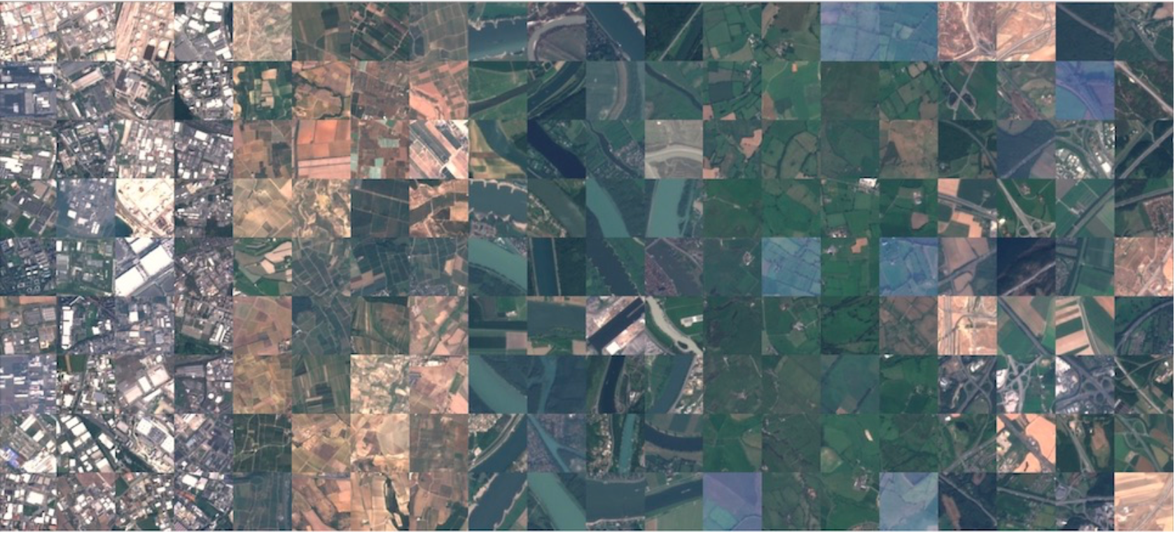
EuroSAT is a Sentinel-2 satellite image benchmark covering 10 land-use/land-cover classes across Europe. This project works through four progressively more capable model families — traditional ML, fully connected networks, CNNs, and multispectral transfer learning — to understand what actually drives classification performance on remote sensing imagery.
Classes: Annual Crop · Forest · Herbaceous Vegetation · Highway · Industrial · Pasture · Permanent Crop · Residential · River · Sea/Lake
1. Data Preparation
EuroSAT RGB patches (64×64 px) were loaded into NumPy arrays. After data augmentation applied before the train/test split, the full dataset contained 81,000 images. A 60/40 stratified split was applied, preserving class proportions across both sets.
| Split | Samples |
|---|---|
| Train | 48,600 |
| Test | 32,400 |
For traditional ML experiments, images were converted to grayscale and flattened into a 2D feature matrix (n × 4096). RGB arrays were kept intact for deep learning.
2. Traditional Machine Learning
Experiments in this section were restricted to three classes: Forest, Residential, and Industrial to enable direct comparison between binary and multiclass approaches under the same flattened grayscale representation.
2.1 Binary SVMs
Three one-vs-one linear SVMs were trained independently:
| Pair | Accuracy | AUC |
|---|---|---|
| Forest vs Residential | 0.9469 | 0.9939 |
| Forest vs Industrial | 0.9973 | 1.0000 |
| Residential vs Industrial | 0.6783 | 0.7257 |
Forest was easy to separate from both built-up classes. Residential vs Industrial proved hardest — in grayscale, these categories share similar texture and spatial density patterns.
2.2 Majority-Vote Multiclass SVM
The three binary classifiers were combined through hard majority voting with soft-score tie-breaking to remove class-order bias.
Multiclass accuracy: 0.769
2.3 Random Forest
A Random Forest trained on the same three-class grayscale data substantially outperformed the SVM ensemble, suggesting non-linear decision boundaries are better suited to this representation.
| Class | Precision | Recall | F1 |
|---|---|---|---|
| Forest | 0.99 | 0.99 | 0.99 |
| Residential | 0.90 | 0.88 | 0.89 |
| Industrial | 0.88 | 0.90 | 0.89 |
| Overall accuracy | 0.9245 |
Residential and Industrial remain the primary confusion pair — a pattern that persists across all model families in this project.
3. Deep Learning
3.1 Fully Connected Networks on Grayscale (10 classes)
Moving to all 10 classes, three fully connected architectures were trained on flattened grayscale pixels.
| Model | Architecture | Parameters | Test Accuracy |
|---|---|---|---|
| Model 1 | Single layer → softmax | 40,970 | 0.1786 |
| Model 2 | Two-layer NN | 1,051,402 | 0.1741 |
| Model 3 | Four-layer NN + dropout | 2,263,178 | 0.1594 |
| Ensemble | Probability avg of 1–3 | — | 0.2103 |
All three models hovered just above the random baseline of 0.10. Adding more depth and parameters made no meaningful difference.
Why? Two compounding problems: (1) flattening destroys spatial structure — edges, texture, and field boundaries that define land cover become unrecoverable from a pixel vector; (2) grayscale removes spectral hue, which is critical for distinguishing water, vegetation, and crop classes. This is a representational mismatch, not a tuning problem.
3.2 CNNs and Transfer Learning on RGB (10 classes)
Switching to convolutional architectures on RGB images produced a dramatic improvement.
| Model | Architecture | Test Accuracy |
|---|---|---|
| Model 4 | Custom CNN (RGB) | 0.8263 |
| Model 5 | MobileNetV2 transfer learning | 0.8793 |
The custom CNN’s +65 percentage point jump over the best fully connected model confirms that spatial locality — preserved by convolution — is the key ingredient for this task. MobileNetV2’s pretrained ImageNet features add another ~5 points even though EuroSAT imagery differs substantially from natural photos.
Remaining errors concentrate in spectrally similar classes: AnnualCrop, PermanentCrop, HerbaceousVegetation, and Pasture are frequently confused. Water bodies and built-up classes are well separated.
3.3 Multispectral Transfer Learning (10 classes)
The best RGB strategy (MobileNetV2 transfer learning) was extended to multispectral input by adding a learnable 4-to-3 channel projection layer before the pretrained backbone. This preserves additional near-infrared spectral information while reusing pretrained visual features.
Training used a two-stage approach: backbone frozen in Stage 1 (projection + head adapts), then final backbone layers unfrozen and fine-tuned in Stage 2 with a lower learning rate and early stopping.
| Model | Test Accuracy |
|---|---|
| Best RGB (MobileNetV2) | 0.8793 |
| Multispectral transfer | 0.9622 |
A +8.3 point improvement from adding a single near-infrared band. The result confirms that spectral information beyond visible RGB carries strong discriminative signal for land-cover classification — consistent with the broader remote sensing literature.
4. Results Summary
| Approach | Scope | Best Accuracy |
|---|---|---|
| Binary SVM | 3 classes, grayscale | 0.9973 (F vs I) |
| Random Forest | 3 classes, grayscale | 0.9245 |
| Fully connected NN | 10 classes, grayscale | 0.2103 (ensemble) |
| Custom CNN | 10 classes, RGB | 0.8263 |
| MobileNetV2 transfer | 10 classes, RGB | 0.8793 |
| Multispectral transfer | 10 classes, RGB+NIR | 0.9622 |
Three things drive performance here: spatial locality (CNNs over dense layers), color/spectral information (RGB over grayscale), and pretrained features + spectral depth (multispectral transfer over custom CNN).